Relaxed Spatial Matching

Inspired by pyramid matching and Hough transform we present a relaxed and flexible spatial matching model which applies the concept of pyramid match to the transformation space. It is invariant to similarity transformations and free of inlier-count verification. Being linear in the number of correspondences, it is fast enough to be used for re-ranking in large scale image retrieval. It imposes one-to-one mapping and is flexible, allowing non-rigid motion and multiple matching surfaces or objects. We compare our proposed algorithm Hough Pyramid Matching (HPM) with the state-of-the Fast Spatial Matching (FSM) for re-ranking top matching images in large scale image retrieval. We show that HPM has superior performance while it is able to re-rank an order of magnitude more images than FSM in the same amount of time.

An image is assumed to be represented by a set of local features, and for each feature we are given its descriptor, position and local shape. We restrict discussion to scale and rotation covariant features. Given two images, an assignment or correspondence is a pair of features betweem the two images and the relative transformation is a similarity transformation. This is a 4-dof transformation represented by a parameter vector $f(c) = (x(c), y(c), \sigma(c), \theta(c))$ and correspondences can be seen as points in a 4-dimensional space. An initial set of candidate or tentative correspondences is constructed according to proximity of features in the descriptor space. Here we consider the simplest visual codebook approach where two features correspond when assigned to the same visual word.

We construct a hierarchical partition of the transformation space into $L$ levels. Each partition of level $\ell$ partitions space into $2^{4(L-\ell-1)}$ bins (hypercubes). The bins are obtained by uniformly quantizing each parameter. We recursively split correspondences into bins in a topdown fashion, and then group them again recursively in a bottom-up fashion. We expect to find most groups of consistent correspondences at the finest (bottom) levels, but we do go all the way up the hierarchy to account for flexibility. Large groups of correspondences formed at a fine level are more likely to be true, or inliers. It follows that each correspondence should contribute to the similarity score according to the size of the groups it participates in and the level at which these groups were formed. In order to impose a one-to-one mapping constraint, we detect conflicting correspondences at each level and greedily choose the best one to keep on our way up the hierarchy. The remaining are marked as erased.

A toy example of the matching process is illustrated in Figures 1, 2, 3. We assume that assignments are conflicting when they share the same visual word, as denoted by color. Three groups of assignments are formed at level $0$: $\{c_1, c_2, c_3\}$, $\{c_4, c_5\}$ and $\{c_6, c_9\}$. The first two are then joined at level 1. Assignments $c_7, c_8$ are conflicting, and $c_7$ is erased at random. Assignments $c_5, c_6$ are also conflicting, but are only compared at level 2 where they share the same bin; $c_5$ is stronger because it participates in a group of 5. Hence group $\{c_6, c_9\}$ is broken up, $c_6$ is erased and finally $c_8, c_9$ join $c_1, \ldots, c_5$ in a group of 7 at level 2. Apart from the feature/assignment configuration in the two images, Figure 2 also illustrates how the similarity score is formed from individual assignment strengths. For instance, assignments $c_1, \ldots, c_5$ have strength contributions from all $3$ levels, while $c_8, c_9$ only from level $2$. Figure 3 shows how these contributions are arranged in a (theoretical) $n \times n$ affinity matrix $A$. In fact, the sum over a row of $A$ equals the strength of the corresponding assignment---note though that the diagonal is excluded. Weights $w(c)$ are related with the initial correspondences; we use the inverse document frequency (idf) of the visual word.

Figure 1. Matching of 9 assignments on a 3-level pyramid in 2D space. Colors denote visual words, and edge strength denotes affinity. There are two pairs of conflicting assignments: c7 is erased at random at level 0, but c5; c6 are only compared at level 2. The one participating in the largest group is kept, that is c5. The dotted line between c6; c9 denotes a group that is formed at level 0 and then broken up at level 2, since c6 is erased.

Figure 2. Assignment labels, colors, features and scores referring to the example of Fig. 1. Note that here vertices and edges denote features and assignments, respectively. Assignments c5; c6 are coflicting, being of the form (p; q); (p; q'). Similarly for c7; c8. Assignments c1,...,c5 join groups at level 0; c8, c9 at level 2; and c6, c7 are erased.

Figure 3.Affinity matrix equivalent to the strengths of Fig. 2. Assignments have been rearranged so that groups appear in contiguous blocks. Groups formed at levels 0, 1, 2 are assigned affinity 1, 1/2, 1/4 respectively. Note that the similarity scores of Fig. 2 may be obtained by summing affinities over rows and multiplying by assignment weights. Assignments are placed on the diagonal, which is excluded from summation.

Here we match two real images of the same scene from different viewpoints. All tentative correspondences are shown, but colored according to the strength they have acquired through the matching process. There are a few mistakes, which is expected since HPM is really a fast approximation. However, it is clear that the strongest correspondences, contributing most to the similarity score, are true inliers. The 3D scene geometry is such that not even a homography can capture the motion of all visible surfaces/objects. Indeed, the inliers to an affine model with FSM are only a small percentage of the initial assignmets. HPM takes no more than 0.6ms to match this particular pair of images, given the features, visual words, and tentative correspondences, while FSM takes about 7ms. Both buildings are matched by HPM, while inliers from one surface are only found by FSM.

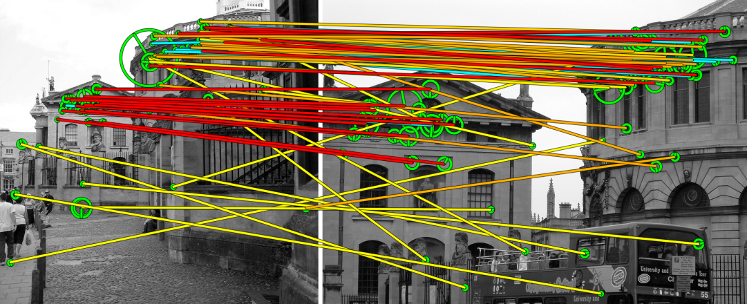
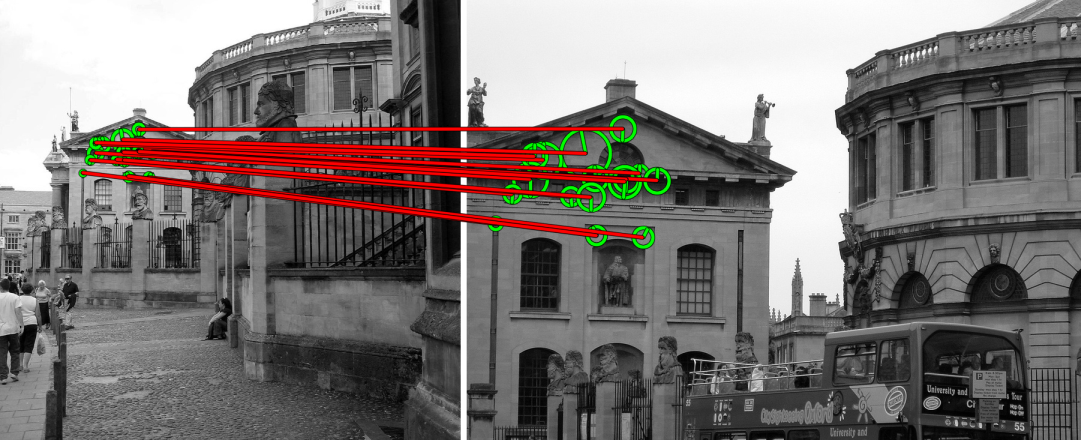
Figure 4. Left: HPM matching of two real images from the Oxford dataset. All tentative correspondences are shown. The ones in cyan have been erased. The rest are colored according to strength, with red (yellow) being the strongest (weakest). Right: Inliers found by 4-dof FSM and affine-model LO-RANSAC.

Figure 5. Correspondences of the example in Figure 4 as votes in 4D transformation space. Two 2D projections are depicted, separately for translation ($x, y$) (zoomed) and log-scale / orientation ($\log \sigma, \theta$). Translation is normalized by maximum image dimension. Maximum scale is set to 10 and orientation shifted by 5$\pi$/16. There are $L$=5 levels. Edges represent links between assignments that are grouped in levels 0,1,2 only. Level affinity $\alpha$ is represented by three tones of gray with black corresponding to $\alpha$(0) = 1.

In analogy to the toy example, Figure 5 illustrates matching of assignments in the Hough space. Observe how assignments get stronger and contribute more by grouping according to proximity, which is a form of consensus.

In order to fit into memory all the information required for each local feature, we quantize each local feature parameter with 5 levels; each parameter is quantized into 16 bins. In our experiments we show that using exactly 5 levels makes sense considering performance and also saves space. Our space requirements per feature, as summarized in Table 1 and are exactly the same as the ones of Weak Geometric Consistency (WGC). Query feature parameters are not quantized.

Table 1. Inverted file memory usage per local feature, in bits. We use run-length encoding for image id, so 2 bytes are sufficient.

We have conducted experiments on two publicly available datasets, namely Oxford Buildings and Paris dataset, as well as on our own World Cities dataset. From the World Cities distractor set we have excluded images from Paris and Barcelona. The former because we also experimented using the publicly available Paris dataset and the latter because the World Cities test set is from Barcelona. Finally the distractor set used in our paper contains about 2M images. More information can be found in the dataset page. We evaluate HPM against state of the art fast spatial matching (FSM) in pairwise matching and in re-ranking in large scale search. In the latter case, we experiment on two filtering models, namely baseline bag-of-words (BoW) and weak geometric consistency (WGC). In all experiments presented here a generic vocabulary of size 100,000 has been used.

Large scale experiments

Figure 6 compares HPM to FSM and baseline, for a varying number of distractors up to 2M. Both BoW and WGC are used for the filtering stage and as baseline. HPM turns out to outperform FSM in all cases. We also re-rank 10K images with HPM, since this takes less time than 1K with FSM. This yields the best performance, especially in the presence of distractors. Interestingly, filtering with BoW or WGC makes no difference in this case. Varying the number of re-ranked images, we measure mAP and query time for FSM and HPM. Once more, we consider both BoW and WGC for filtering. A combined plot is given in Figure 7. HPM appears to re-rank ten times more images in less time than FSM. With BoW, its mAP is 10% higher than FSM for the same re-ranking time, on average. At the price of 7 additional seconds for filtering, FSM eventually benefits from WGC, while HPM is clearly unaffected. Indeed, after about 3.3 seconds, mAP performance of BoW+HPM reaches \emph{saturation} after re-ranking 7K images, while WGC does not appear to help.

Figure 6. mAP comparison for varying database size on World Cities dataset with up to 2M distractors. Filtering is performed with BoW or WGC and re-ranking top 1K with FSM or HPM, except HPM10K, where BoW and WGC curves coincide.	Figure 7. mAP and total (filtering + re-ranking) query time for a varying number of re-ranked images. The latter are shown with text labels near markers, in thousands. Results on the World Cities dataset with 2M distractors.

We present retrieval examples for differents methods on the World Cities dataset with 2M distractors. Compared methods are BoW, BoW with FSM for re-ranking top 1000 images, BoW with HPM for re-ranking top 1000 images and BoW with HPM for re-ranking top 10000 images. Top 40 retrieved images are shown. All ground-truth images depicting the same object as the particular query image are 73.

BoW, average precision: 0.026, query time: 282 ms
BoW and re-ranking top 1000 with Fast Spatial Matching, average precision: 0.117, query time: 5054 ms
BoW and re-ranking top 1000 with Hough Pyramid Matching, average precision: 0.156, query time: 976 ms
BoW and re-ranking top 10000 with Hough Pyramid Matching, average precision: 0.504, query time: 4350 ms

We have developed a very simple spatial matching algorithm that requires no learning and can be easily implemented and integrated in any visual search engine. It boosts performance by allowing flexible matching. Following the previous discussion, this boost is expected to come in addition to benefits from e.g. codebook enhancements or query expansion. It is arguably the first time a spatial re-ranking method reaches its saturation in as few as 3 seconds.

Binary code for image retrieval with HPM can be found here.

The proposed HPM algorithm is integrated in an experimental retrieval demo used for automatic location estimation and landmark recognition. This is an experimental version of the VIRaL search engine. VIRaL uses FSM to re-rank top 100 images, while the experimental demo uses HPM to re-rank top 1000 images. Comparisons can be made for the same query images between the two systems. However note that there are differences, such as that FSM uses 3 nearest visual words for query image features but HPM only 1. HPM is tested under large scale retrieval experiments and is proved to increase mean Average Precision. In the application of location estimation and landmark recognition using a strict threshold and providing only true results is a desirable property. HPM is not yet tested and tuned to perform in this way.